Details on OMx Methods

Details about theory and implementation of up-to-now most advanced semiempirical quantum-chemical methods are published.

Semiempirical quantum-chemical (SQC) methods were a major tool for computational chemists for a long time. Then spurred by the advances in computer technology, theoreticians largely concentrated on development and application of ab initio and DFT methods, while inherently much faster SQC techniques were in this regard somewhat neglected. Still, SQC techniques bridge the gap between molecular mechanics (MM) and DFT methods both in terms of speed and accuracy and are therefore indispensable for many applications. Moreover, for many applications accuracy of SQC methods is comparable or even exceed the accuracy of common DFT methods as in this study. Thus, I often use SQC methods in my research.

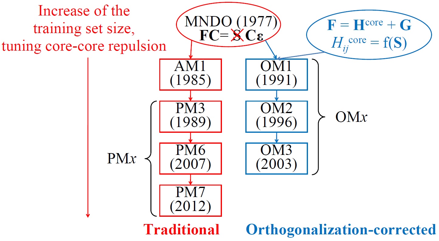
The family of the most widely used SQC methods has two main lines: traditional and orthogonalization-corrected (OMx) methods. Traditional ones build on the parent MNDO model and thus sometimes called MNDO-type, MNDO-like, or MNDO-based method. The general idea behind them is to use the original MNDO model and improve it by extensive parametrization and by modifying core-repulsion functions. Examples include popular and quite accurate PM6 and PM7 methods.

Thiel’s OMx methods go beyond MNDO model as they include explicitly orthogonalization corrections formally neglected in MNDO-type methods. In addition to the repulsive orthogonalization corrections \(V^\text{ORT}\) OMx methods include attractive penetration integrals \(V^\text{PI}\) and repulsive effective core potentials \(V^\text{ECP}\) [1]:

$$  H_{\mu\nu}^\text{core} =  U_{\mu\mu}\delta_{\mu\nu} +  \sum_{B} \left[      V_{\mu\nu,B}^\text{s}    + V_{\mu\nu,B}^\text{ORT}    + V_{\mu\nu,B}^\text{PI}    + V_{\mu\nu,B}^\text{ECP}    \right]\label{eqn:Hcore-mu-nu} $$
$$  H_{\mu\lambda}^\text{core} =   \beta_{\mu\lambda} +  \sum_{C} V_{\mu\lambda,C}^\text{ORT}$$

These changes affect only the core-Hamiltonian. As a result of an improved physical model of OMx methods compared to MNDO-type methods, the former ones excel in accuracy in both ground- and excited-state calculations [1].

Three variants of OMx methods exist: OM1, OM2, and OM3. Apart from different parameter sets, their major formal distinction is in the extend to which orthogonalization corrections are included:

$$  V_{\mu\nu,B}^\text{ORT} = -\frac{1}{2}F_{1}^\text{A}\sum_{\rho \in B}   \left(S_{\mu\rho}\beta_{\rho\nu} + \beta_{\mu\rho}S_{\rho\nu}\right) +\frac{1}{8}F_{2}^\text{A}\sum_{\rho \in B}   S_{\mu\rho}S_{\rho\nu}  \left(H_{\mu\mu,B}^\text{loc} + H_{\nu\nu,B}^\text{loc} – 2H_{\rho\rho,A}^\text{loc}\right)\label{eqn:V-ORT-two} $$
$$  V_{\mu\lambda,C}^\text{ORT} = -\frac{1}{2}G_{1}^\text{AB}\sum_{\rho \in C}   \left(S_{\mu\rho}\beta_{\rho\lambda} + \beta_{\mu\rho}S_{\rho\lambda}\right) $$

$$+\frac{1}{8}G_{2}^\text{AB}\sum_{\rho \in C}   S_{\mu\rho}S_{\rho\lambda}
\left(H_{\mu\mu,C}^\text{loc} + H_{\lambda\lambda,C}^\text{loc} – H_{\rho\rho,A}^\text{loc} – H_{\rho\rho,B}^\text{loc}\right) $$

OM2 include all above terms, while OM1 includes only \(V_{\mu\nu,B}^\text{ORT}\) and OM3 neglects second-order terms, i.e. sets \(F_2 = 0\) and \(G_2 = 0\). OM2 is therefore the slowest method, but still its speed is comparable with MNDO-type methods [1].

In the paper [1] we finally provide complete and concise description of OMx methods together with their parameters. Early, description of OM2 and OM3 was only available in several voluminous PhD theses in German. In addition, we present validation and comparison with other SQC methods for the training set of OMx methods (for extensive benchmark on other sets, see our accompanying paper).

One of the remaining drawbacks of OMx methods is that similarly to DFT methods they do not describe well dispersion interactions. Luckily for us Stefan Grimme has done an excellent job with his D2 (re-parametrized by Xin Wu for OM2 and OM3 [1]) and D3 corrections (with parameters fitted by Risthaus and Grimme for OM2 and OM3). Thus, we also briefly discuss resulting OMx-Dn methods [1].

There is still a wiggle room to improve OMx methods. One of them is to extend their parametrization to elements other than H, C, N, O, and F. On this note, I believe that in future we’ll see around more improvements of SQC methods by traditional means as well as using novel approaches. As for the latter ones, check our efforts on improving SQC methods with machine learning.

1. Pavlo O. Dral, Xin Wu, Lasse Spörkel, Axel Koslowski, Wolfgang Weber, Rainer Steiger, Mirjam Scholten, Walter Thiel, Semiempirical Quantum-Chemical Orthogonalization-Corrected Methods: Theory, Implementation, and Parameters. J. Chem. Theory Comput. 2016, ASAP. DOI: 10.1021/acs.jctc.5b01046.